Announcements

• Midterm is next week

  • Please be on time!
  • Make sure HonorLock works without problems.
  • Check the course website for recommendations.

• Answer key for Homework 3 is posted on the course website.

• Review session for the midterm on Friday 2.00pm at UTC 3.102

• Check out the answers for the JITTs on the course website:

  • Even if you got full credit, check the feedback and the correct answer.

Last class

Today

Another identification strategy

RCTs

Selection on observables

Natural experiments

Difference-in-Differences

Regression Discontinuity Designs

Tell me something about the readings/videos you had to watch for this week

Introduction to Regression Discontinuity Designs

Regression Discontinuity (RD) Designs

Arbitrary rules determine treatment assignment

E.g.: If you are above a threshold, you are assigned to treatment, and if your below, you are not (or vice versa)

Geographic discontinuities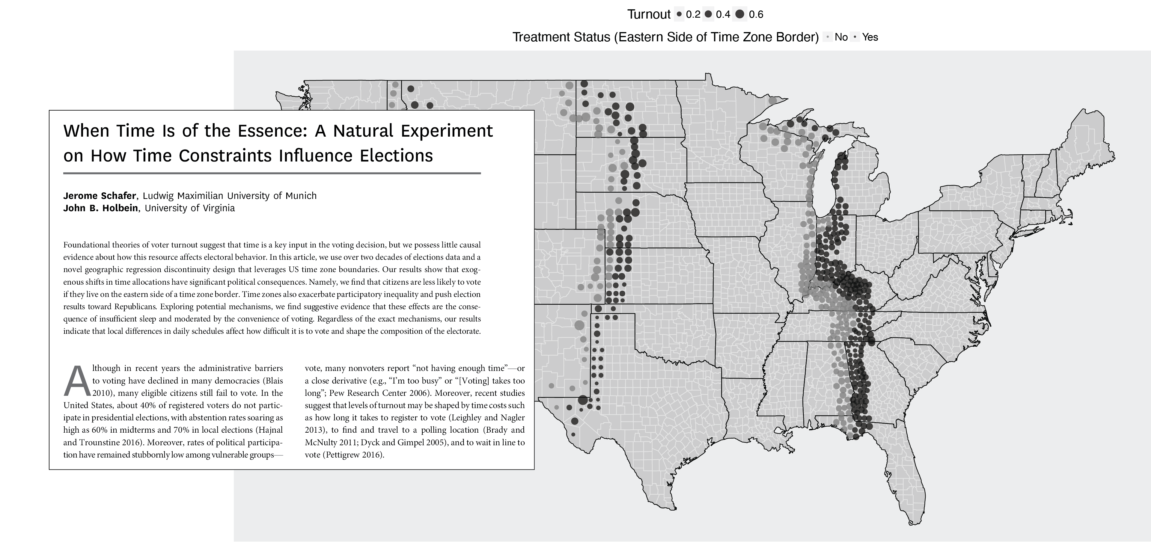

Time discontinuities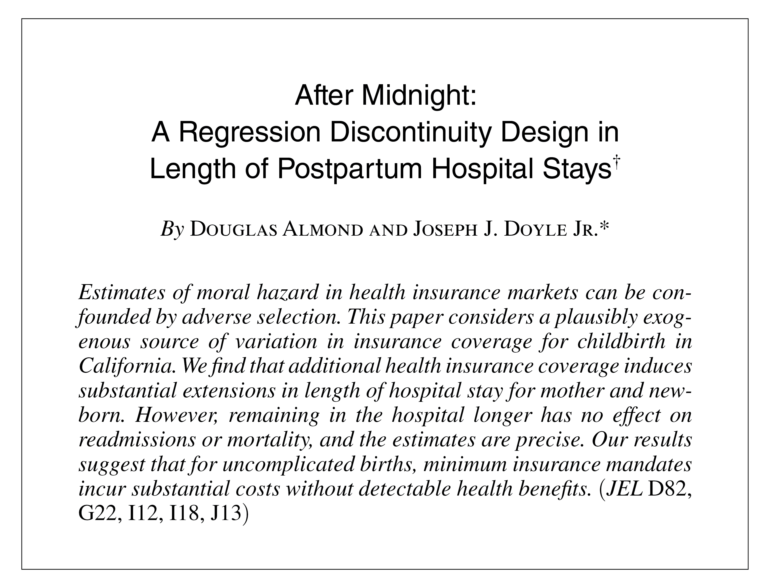

Voting discontinuities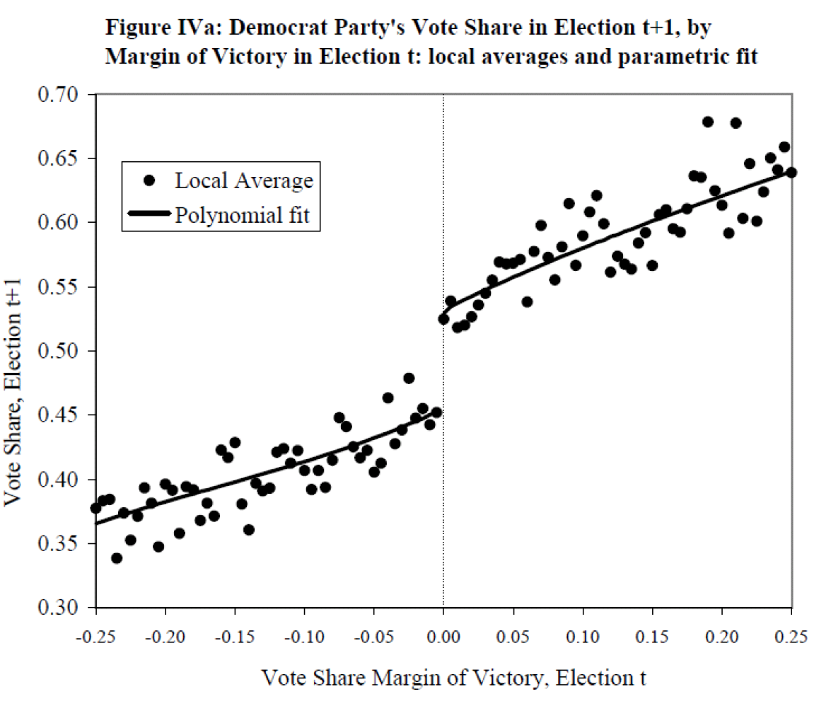

Key Terms

Running/ forcing variable

Index or measure that determines eligibility

Cutoff/ cutpoint/ threshold

Number that formally assigns you to a program or treatment

Let's look at an example

Hypothetical tutoring program

Students take an entrance exam

Those who score 70 or lower
get a free tutor for the year

Students then take an exit exam
at the end of the year

Assignment based on entrance score

Let's look at the area close to the cutoff

Let's get closer

Causal inference intuition

Observations right before and after the threshold are essentially the same

Pseudo treatment and control groups!

Compare outcomes right at the cutoff

Exit exam results according to running variable

Fit a regression at the right and left side of the cutoff

Fit a regression at the right and left side of the cutoff

Is that what we want?

Probably not ideal, there may not be any units with R=c

... but better LATE than nothing!

Conditions required for identification

• Threshold rule exists and cutoff point is known

  • There needs to be a discontinuity in treatment assignment, and we need to know where it happens!

• The running variable $R_i$ is continuous near $c$.

  • If we are working with a coarse variable, this might not work.

• Key assumption:

Continuity of E[Y(1)|R] and E[Y(0)|R] at R=c

That's the math-y way to say that the only thing that changes right at the cutoff is the treatment assignment!

We need to identify that "jump"

How do we actually estimate an RDD?

• The simplest way to do this is to fit a regression using an interaction of the treatment variable and the running variable:

$$Y={\beta }_0+{\beta }_1(R-c)+{\beta }_{2}I[R>c]+{\beta }_3(R-c)I[R>c]+\epsilon$$

How do we actually estimate an RDD?

• The simplest way to do this is to fit a regression using an interaction of the treatment variable and the running variable:

$$Y={\beta }_0+{\beta }_1\underset{\text{Distance to the cutoff}}{\underset{}{(R-c)}}+{\beta }_2\underset{\text{Treatment}}{\underset{}{I[R>c]}}+{\beta }_3\stackrel{\text{Distance to the cutoff}}{\stackrel{}{(R-c)}}\underset{\text{Treatment}}{\underset{}{I[R>c]}}+\epsilon$$

• We can simplify this with new notation:

$$Y_i={\beta }_0+{\beta }_1{R}^{\prime }+{\beta }_{2}Treat+{\beta }_3{R}^{\prime }\times Treat$$

where $Treat$ is a binary treatment variable and $R^{\prime }$ is the running variable centered around the cutoff

Can you identify these parameters in a plot?

Let's identify coefficients

Steps for analyzing an RDD

1) Check that there is a discontinuity in treatment assignment at the cutoff.

2) Check that covariates change smoothly across the threshold.

• You can think about this as the equivalent of a balance table.

3) Run the regression discontinuity design model.

• Interpret this effect for individuals right at the cutoff.

Discount and sales

Discounts and sales: Data available

• We have the following dataset, with time of arrival for customers, a few covariates, and the outcome of interest (sales)

sales = read.csv("https://raw.githubusercontent.com/maibennett/sta235/main/exampleSite/content/Classes/Week8/1_RDD/data/sales.csv")
head(sales)

##   id     time age female   income    sales treat
## 1  1 1.050000  49      1 83622.63 231.0863     1
## 2  2 1.203883  50      1 67265.61 215.6148     1
## 3  3 1.332719  46      1 59151.46 200.5003     1
## 4  4 1.608881  49      0 67308.17 203.9145     1
## 5  5 1.637072  50      1 65420.20 217.6668     1
## 6  6 1.871347  47      0 68566.67 222.0601     1

Discounts and sales: Can we use an RDD?

• In RDD, we need to check that there are no unbalances in covariates across the threshold.

sales = sales %>% mutate(dist = c-time)
lm(income ~ dist*treat, data = sales)

RDD on sales using linear models

lm(sales ~ dist*treat, data = sales)

RDD on sales using linear models

summary(lm(sales ~ dist*treat, data = sales))

## 
## Call:
## lm(formula = sales ~ dist * treat, data = sales)
## 
## Residuals:
##     Min      1Q  Median      3Q     Max 
## -65.738 -13.940   0.051  13.538  76.515 
## 
## Coefficients:
##               Estimate Std. Error t value Pr(>|t|)    
## (Intercept) 178.640954   1.300314  137.38   <2e-16 ***
## dist          0.205355   0.008882   23.12   <2e-16 ***
## treat        31.333952   1.842338   17.01   <2e-16 ***
## dist:treat   -0.200845   0.012438  -16.15   <2e-16 ***
## ---
## Signif. codes:  0 '***' 0.001 '**' 0.01 '*' 0.05 '.' 0.1 ' ' 1
## 
## Residual standard error: 20.52 on 1996 degrees of freedom
## Multiple R-squared:  0.6939,    Adjusted R-squared:  0.6934 
## F-statistic:  1508 on 3 and 1996 DF,  p-value: < 2.2e-16

On average, providing a 10% discount increases sales by $31.3 for the 1,000 customer, compared to not having a discount

We can be more flexible

• The previous example just included linear terms, but you can also be more flexible:

$$Y={\beta }_0+{\beta }_{1}f\left(R^{\prime }\right)+{\beta }_{2}Treat+{\beta }_{3}f\left(R^{\prime }\right)\times Treat+\epsilon$$

• Where $f$ is any function you want.

What happens if we fit a quadratic model?

lm(sales ~ dist*treat + treat*I(dist^2), data = sales)

What happens if we fit a quadratic model?

summary(lm(sales ~ dist*treat + treat*I(dist^2), data = sales))

## 
## Call:
## lm(formula = sales ~ dist * treat + treat * I(dist^2), data = sales)
## 
## Residuals:
##     Min      1Q  Median      3Q     Max 
## -66.090 -13.979   0.239  13.154  76.656 
## 
## Coefficients:
##                   Estimate Std. Error t value Pr(>|t|)    
## (Intercept)      1.698e+02  1.937e+00  87.665  < 2e-16 ***
## dist            -4.302e-03  3.556e-02  -0.121 0.903725    
## treat            3.308e+01  2.747e+00  12.041  < 2e-16 ***
## I(dist^2)       -8.288e-04  1.363e-04  -6.083 1.41e-09 ***
## dist:treat       1.713e-01  4.964e-02   3.452 0.000569 ***
## treat:I(dist^2)  2.034e-04  1.877e-04   1.084 0.278554    
## ---
## Signif. codes:  0 '***' 0.001 '**' 0.01 '*' 0.05 '.' 0.1 ' ' 1
## 
## Residual standard error: 20.23 on 1994 degrees of freedom
## Multiple R-squared:  0.7029,    Adjusted R-squared:  0.7021 
## F-statistic: 943.5 on 5 and 1994 DF,  p-value: < 2.2e-16

On average, providing a 10% discount increases sales by $33.1 for the 1,000 customer, compared to not having a discount

What happens if we only look at observations close to c?

sales_close = sales %>% filter(dist>-100 & dist<100)
lm(sales ~ dist*treat, data = sales_close)

How do they compare?

summary(lm(sales ~ dist*treat, data = sales_close))

## 
## Call:
## lm(formula = sales ~ dist * treat, data = sales_close)
## 
## Residuals:
##     Min      1Q  Median      3Q     Max 
## -53.241 -14.764   0.268  12.938  57.811 
## 
## Coefficients:
##              Estimate Std. Error t value Pr(>|t|)    
## (Intercept) 170.84457    2.05528  83.125   <2e-16 ***
## dist          0.06345    0.03542   1.791   0.0736 .  
## treat        32.21243    2.93614  10.971   <2e-16 ***
## dist:treat    0.06909    0.05047   1.369   0.1714    
## ---
## Signif. codes:  0 '***' 0.001 '**' 0.01 '*' 0.05 '.' 0.1 ' ' 1
## 
## Residual standard error: 20.25 on 782 degrees of freedom
## Multiple R-squared:  0.5261,    Adjusted R-squared:  0.5243 
## F-statistic: 289.4 on 3 and 782 DF,  p-value: < 2.2e-16

On average, providing a 10% discount increases sales by $32.2 for the 1,000 customer, compared to not having a discount

Potential problems

• There are many potential problems with the previous examples:

  • Which polynomial function should we choose? Linear, quadratic, other?

  • What bandwidth should we choose? Whole sample? [-100,100]?

• There are some ways to address these concerns.

Package rdrobust

• Robust Regression Discontinuity introduced by Cattaneo, Calonico, Farrell & Titiunik (2014).

• Use of local polynomial for fit.

• Data-driven optimal bandwidth (bias vs variance).

• rdrobust: Estimation of LATE and opt. bandwidth

• rdplot: Plotting RD with nonparametric local polynomial.

Let's compare with previous parametric results

rdplot(y = sales$sales, x = sales$dist, c = 0, 
       title = "RD plot", x.label = "Time to 1,000 customer (min)", y.label = "Sales ($)")

Let's compare with previous parametric results

rdplot(y = sales$sales, x = sales$dist, c = 0, 
       title = "RD plot", x.label = "Time to 1,000 customer (min)", y.label = "Sales ($)")

Let's compare with previous parametric results

rd_sales = rdrobust(y = sales$sales, x = sales$dist, c = 0)
summary(rd_sales)

## Sharp RD estimates using local polynomial regression.
## 
## Number of Obs.                 2000
## BW type                       mserd
## Kernel                   Triangular
## VCE method                       NN
## 
## Number of Obs.                 1000         1000
## Eff. Number of Obs.             209          200
## Order est. (p)                    1            1
## Order bias  (q)                   2            2
## BW est. (h)                  53.578       53.578
## BW bias (b)                  87.522       87.522
## rho (h/b)                     0.612        0.612
## Unique Obs.                    1000         1000
## 
## =============================================================================
##         Method     Coef. Std. Err.         z     P>|z|      [ 95% C.I. ]       
## =============================================================================
##   Conventional    37.772     4.370     8.644     0.000    [29.208 , 46.336]    
##         Robust         -         -     7.684     0.000    [29.124 , 49.070]    
## =============================================================================

Takeaway points

References

• Angrist, J. and S. Pischke. (2015). "Mastering Metrics". Chapter 4.

• Social Science Research Institute at Duke University. (2015). “Regression Discontinuity: Looking at People on the Edge: Causal Inference Bootcamp”