Introduction to Rmarkdown
Here are some resources so you get an introduction to Rmarkdown. This introduction just consolidates material from “R Markdown: The Definitive Guide” (2021) by Yihui Xie, J. J. Allaire, and Garrett Grolemund, and also Andrew Heiss’ awesome instructional website. All credit goes to them.
In this tutorial, the topics covered are:
Installation Requirements
You will need to have the following programs and packages installed on your laptop:
Once you have both software installed, go into RStudio and install the following packages:
-
The package
rmarkdown: Typeinstall.packages("rmarkdown") -
The package
tinytex: Following these instructions, typeinstall.packages("tinytex")(and hit enter), and then typetinytex::install_tinytex()
You need tinytex (or another LaTeX program) to be able to knit (compile) your Rmarkdown files into PDFs. PS: By the way, it’s pronounced “lay-tek”. Not sure why.
Using Markdown
All material and resources in the following sections were created by Andrew Heiss.
Markdown is a special kind of markup language that lets you format text with simple syntax. You can then use a converter program like pandoc to convert Markdown into whatever format you want: HTML, PDF, Word, PowerPoint, etc. We will be using specifically Rmarkdown, which is just a markdown file that combines R code as well.
Basic Markdown formatting
| Type… | …or… | …to get |
|---|---|---|
Some text in a paragraph. |
Some text in a paragraph. More text in the next paragraph. Always use empty lines between paragraphs. |
|
*Italic* |
_Italic_ |
Italic |
**Bold** |
__Bold__ |
Bold |
# Heading 1 |
Heading 1 |
|
## Heading 2 |
Heading 2 |
|
### Heading 3 |
Heading 3 |
|
(Go up to heading level 6 with ######) |
||
[Link text](http://www.example.com) |
Link text | |
 |
 |
|
`Inline code` with backticks |
Inline code with backticks |
|
> Blockquote |
|
|
- Things in - an unordered - list |
* Things in * an unordered * list |
|
1. Things in 2. an ordered 3. list |
1) Things in 2) an ordered 3) list |
|
Horizontal line |
Horizontal line |
Horizontal line |
Math
Markdown uses LaTeX to create fancy mathematical equations. There are like a billion little options and features available for math equations—you can find helpful examples of the the most common basic commands here.
You can use math in two different ways: inline or in a display block. To use math inline, wrap it in single dollar signs, like \$y = mx + b\$:
| Type… | …to get |
|---|---|
The regression model for
estimating the effect of education on wages
is $\hat{y} = \beta_0 + \beta_1 x_1 + \epsilon$, or
$\text{Wages} = \beta_0 + \beta_1 \text{Education} + \epsilon$. |
The regression model for estimating the effect of education on wages is \(\hat{y} = \beta_0 + \beta_1 x_1 + \epsilon\), or \(\text{Wages} = \beta_0 + \beta_1 \text{Education} + \epsilon\). |
To put an equation on its own line in a display block, wrap it in double dollar signs, like this:
Type…
The quadratic equation was an important part of high school math:

$$
x = \frac{-b \pm \sqrt{b^2 - 4ac}}{2a}
$$

But now we just use computers to solve for $x$.
…to get…
The quadratic equation was an important part of high school math:
$$ x = \frac{-b \pm \sqrt{b^2 - 4ac}}{2a} $$
But now we just use computers to solve for $x$.
Because dollar signs are used to indicate math equations, you can’t just use dollar signs like normal if you’re writing about actual dollars. For instance, if you write This book costs \$5.75 and this other costs \$40, Markdown will treat everything that comes between the dollar signs as math, like so: “This book costs $5.75 and this other costs $40”.
To get around that, put a backslash (\) in front of the dollar signs, so that This book costs \\\$5.75 and this other costs \\\$40 becomes “This book costs $5.75 and this other costs $40”.
Tables
There are 4 different ways to hand-create tables in Markdown—I say “hand-create” because it’s normally way easier to use R to generate these things with packages like knitr (use kable() or stargazer (see the Rmarkdown template at the end of this tutorial) depending what you are analyzing). The two most common are simple tables and pipe tables. You should look at the full documentation here.
For simple tables, type…
  Right     Left     Center     Default
-------     ------ ----------   -------
     12     12        12            12
    123     123       123          123
      1     1          1             1

Table: Caption goes here
…to get…
Right Left Center Default
 12     12        12            12
123     123       123          123
  1     1          1             1
Table: Caption goes here
For pipe tables, type…
| Right | Left | Default | Center |
|------:|:-----|---------|:------:|
|   12  |  12  |    12   |    12  |
|  123  |  123 |   123   |   123  |
|    1  |    1 |     1   |     1  |

Table: Caption goes here
…to get…
| Right | Left | Default | Center |
|---|---|---|---|
| 12 | 12 | 12 | 12 |
| 123 | 123 | 123 | 123 |
| 1 | 1 | 1 | 1 |
Table: Caption goes here
Footnotes
There are two different ways to add footnotes (see here for complete documentation): regular and inline.
Regular notes need (1) an identifier and (2) the actual note. The identifier can be whatever you want. Some people like to use numbers like [^1], but if you ever rearrange paragraphs or add notes before #1, the numbering will be wrong (in your Markdown file, not in the output; everything will be correct in the output). Because of that, I prefer to use some sort of text label:
Type…
Here is a footnote reference[^1] and here is another [^note-on-dags].

[^1]: This is a note.

[^note-on-dags]: DAGs are neat.

And here's more of the document.
…to get…
Here is a footnote reference1 and here is another.2
And here’s more of the document.
You can also use inline footnotes with ^[Text of the note goes here], which are often easier because you don’t need to worry about identifiers:
Type…
Causal inference is neat.^[But it can be hard too!]
…to get…
Causal inference is neat.1
But it can be hard too!↩︎
Front matter
You can include a special section at the top of a Markdown document that contains metadata (or data about your document) like the title, date, author, etc. This section uses a special simple syntax named YAML (or “YAML Ain’t Markup Language”) that follows this basic outline: setting: value for setting. Here’s an example YAML metadata section. Note that it must start and end with three dashes (---).
---
title: Title of your document
date: "January 13, 2020"
author: "Your name"
---
You can put the values inside quotes (like the date and name in the example above), or you can leave them outside of quotes (like the title in the example above). I typically use quotes just to be safe—if the value you’re using has a colon (:) in it, it’ll confuse Markdown since it’ll be something like title: My cool title: a subtitle, which has two colons. It’s better to do this:
---
title: "My cool title: a subtitle"
---
If you want to use quotes inside one of the values (e.g. your document is An evaluation of "scare quotes"), you can use single quotes instead:
---
title: 'An evaluation of "scare quotes"'
---
Citations
One of the most powerful features of Markdown + pandoc is the ability to automatically cite things and generate bibliographies. to use citations, you need to create a BibTeX file (ends in .bib) that contains a database of the things you want to cite. You can do this with bibliography managers designed to work with BibTeX directly (like BibDesk on macOS), or you can use Zotero (macOS and Windows) to export a .bib file. You can download an example .bib file of all the readings from this class here.
Complete details for using citations can be found here. In brief, you need to do three things:
-
Add a
bibliography:entry to the YAML metadata:--- title: Title of your document date: "January 13, 2020" author: "Your name" bibliography: name_of_file.bib --- -
Choose a citation style based on a CSL file. The default is Chicago author-date, but you can choose from 2,000+ at this repository. Download the CSL file, put it in your project folder, and add an entry to the YAML metadata (or provide a URL to the online version):
---
title: Title of your document
date: "January 13, 2020"
author: "Your name"
bibliography: name_of_file.bib
csl: "https://raw.githubusercontent.com/citation-style-language/styles/master/apa.csl"
---
Some of the most common CSLs are:
- Chicago author-date
- Chicago note-bibliography
- Chicago full note-bibliography (no shortened notes or ibids)
- APA 7th edition
- MLA 8th edition
-
Cite things in your document. Check the documentation for full details of how to do this. Essentially, you use
@citationkeyinside square brackets ([]):
| Type… | …to get |
|---|---|
Causal inference is neat[@Rohrer:2018; @AngristPischke:2015]. |
Causal Inference is neat (Rohrer 2018; Angrist and Pischke 2015). |
Causal inference is neat[see @Rohrer:2018, p. 34; also @AngristPischke:2015, chapter 1]. |
Causal inference is neat (see Rohrer 2018, 34; also Angrist and Pischke 2015, chap. 1). |
Angrist and Pischke say causal inference is neat[-@AngristPischke:2015; see also @Rohrer:2018]. |
Angrist and Pischke say causal inference is neat (2015; see also Rohrer 2018). |
@AngristPischke:2015 [chapter 1] say causal inferenceis neat, and @Rohrer:2018 agrees. |
Angrist and Pischke (2015, chap. 1) say causal inference is neat, and Rohrer (2018) agrees. |
After compiling, you should have a perfectly formatted bibliography added to the end of your document too:
Angrist, Joshua D., and Jörn-Steffen Pischke. 2015. Mastering ’Metrics: The Path from Cause to Effect. Princeton, NJ: Princeton University Press.
Rohrer, Julia M. 2018. “Thinking Clearly About Correlations and Causation: Graphical Causal Models for Observational Data.” Advances in Methods and Practices in Psychological Science 1 (1): 27–42. https://doi.org/10.1177/2515245917745629.
Other references
These websites have additional details and examples and practice tools:
- CommonMark’s Markdown tutorial: A quick interactive Markdown tutorial.
- Markdown tutorial: Another interactive tutorial to practice using Markdown.
- Markdown cheatsheet: Useful one-page reminder of Markdown syntax.
- The Plain Person’s Guide to Plain Text Social Science: A comprehensive explanation and tutorial about why you should write data-based reports in Markdown.
Using RMarkdown
RMarkdown is just regular Markdown but it also includes R code. The advantages is that you can incorporate chunks of code, plots, tables, and all the analysis that you do on R in your write-ups or documents! This is a great way to make reproducible documents.
Key terms
-
Document: A Markdown file where you type stuff
-
Chunk: A piece of R code that is included in your document. It looks like this:
`r ''````{r}
# Code goes here
```
There must be an empty line before and after the chunk. The final three backticks must be the only thing on the line—if you add more text, or if you forget to add the backticks, or accidentally delete the backticks, your document will not knit correctly.
-
Knit: When you “knit” a document, R runs each of the chunks sequentially and converts the output of each chunk into Markdown. R then runs the knitted document through pandoc to convert it to HTML or PDF or Word (or whatever output you’ve selected).
You can knit by clicking on the “Knit” button at the top of the editor window, or by pressing
⌘⇧Kon macOS orcontrol + shift + Kon Windows.
Add chunks
There are three ways to insert chunks:
-
Press
⌘⌥Ion macOS orcontrol + alt + Ion Windows -
Click on the “Insert” button at the top of the editor window
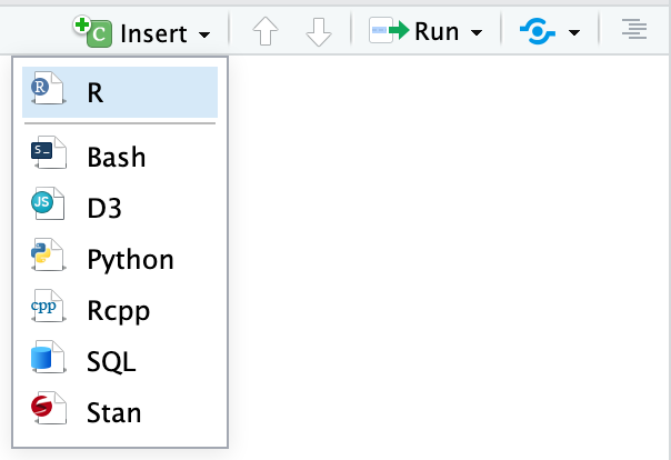
- Manually type all the backticks and curly braces (don’t do this)
Chunk names
You can add names to chunks to make it easier to navigate your document. If you click on the little dropdown menu at the bottom of your editor in RStudio, you can see a table of contents that shows all the headings and chunks. If you name chunks, they’ll appear in the list. If you don’t include a name, the chunk will still show up, but you won’t know what it does.
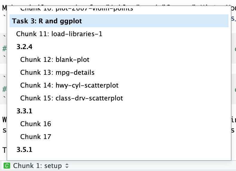
To add a name, include it immediately after the {r in the first line of the chunk. Names cannot contain spaces, but they can contain underscores and dashes. All chunk names in your document must be unique.
`r ''````{r name-of-this-chunk}
# Code goes here
```
Chunk options
There are a bunch of different options you can set for each chunk. You can see a complete list in the RMarkdown Reference Guide or at knitr’s website.
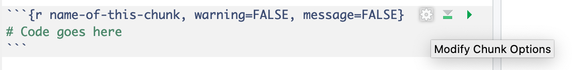
Options go inside the {r} section of the chunk:
`r ''````{r name-of-this-chunk, warning=FALSE, message=FALSE}
# Code goes here
```
The most common chunk options are these:
fig.width=5andfig.height=3(or whatever number you want): Set the dimensions for figuresecho=FALSE: The code is not shown in the final document, but the results aremessage=FALSE: Any messages that R generates (like all the notes that appear after you load a package) are omittedwarning=FALSE: Any warnings that R generates are omittedinclude=FALSE: The chunk still runs, but the code and results are not included in the final document
You can also set chunk options by clicking on the little gear icon in the top right corner of any chunk:
Inline chunks
You can also include R output directly in your text, which is really helpful if you want to report numbers from your analysis. To do this, use `r "\u0060r r_code_here\u0060"`.
It’s generally easiest to calculate numbers in a regular chunk beforehand and then use an inline chunk to display the value in your text. For instance, this document…
`r ''````{r find-avg-mpg, echo=FALSE}
avg_mpg <- mean(mtcars$mpg)
```

The average fuel efficiency for cars from 1974 was `r "\u0060r round(avg_mpg, 1)\u0060"` miles per gallon.
… would knit into this:
The average fuel efficiency for cars from 1974 was
r round(mean(mtcars$mpg), 1)miles per gallon.
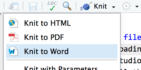
Output formats
You can specify what kind of document you create when you knit in the YAML front matter.
title: "My document"
output:
  html_document: default
  pdf_document: default
  word_document: default
You can also click on the down arrow on the “Knit” button to choose the output and generate the appropriate YAML. If you click on the gear icon next to the “Knit” button and choose “Output options”, you change settings for each specific output type, like default figure dimensions or whether or not a table of contents is included.
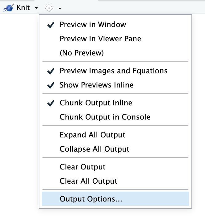
The first output type listed under output: will be what is generated when you click on the “Knit” button or press the keyboard shortcut (⌘⇧K on macOS; control + shift + K on Windows). If you choose a different output with the “Knit” button menu, that output will be moved to the top of the output section.
The indentation of the YAML section matters, especially when you have settings nested under each output type. Here’s what a typical output section might look like:
---
title: "My document"
author: "My name"
date: "January 13, 2020"
output:
  html_document:
    toc: yes
    fig_caption: yes
    fig_height: 8
    fig_width: 10
  pdf_document:
    latex_engine: xelatex  # More modern PDF typesetting engine
    toc: yes
  word_document:
    toc: yes
    fig_caption: yes
    fig_height: 4
    fig_width: 5
---
Other references
- Documentation for Rmarkdown: Extensive guide on everything you need to know about RMarkdown.
- RMarkdown tutorial: Helpful tutorials to learn more about this!
- RMarkdown cheatsheet: Cheatsheets are life.
RMarkdown template
Finally, put your knowledge to the test! Here is a small template you can use to play around and customize however you like it.
View PDF templateDownload template
© Magdalena Bennett - licensed under Creative Commons.